2.1. Difference image decorrelation.¶

An algorithm developed by Kaiser (2004) and later rediscovered by Zackay, et al. (2015) showed that the noise in a PSF-matched coadd image can be decorrelated via noise whitening (i.e. flattening the noise spectrum). The same principle may also be applied to image differencing (Zackay, et al. (2016)). In the case of A&L PSF matching, this results in an image difference in Fourier space \(D(k)\):

Here, \(X(k)\) denotes the FFT of \(X\); \(\overline{\sigma}_i^2\) is the mean of the per-pixel variances of image \(I_i\) – i.e., \(\overline{\sigma}_i^2 = \frac{\sum_{x,y} \sigma_i^2(x,y)}{N_{x,y}}\). Thus, we may perform PSF matching to estimate \(\kappa\) by standard methods (e.g., A&L and related methods) and then correct for the noise in the template via (1). The term in the square-root of (1) is a post-subtraction convolution kernel, or decorrelation kernel \(\psi(k)\),

which is convolved with the image difference, and has the effect of decorrelating the noise in the image difference that was introduced by convolution of \(I_2\) with the A&L PSF matching kernel \(\kappa\). It also (explicitly) contains an extra factor of \(\sqrt{\overline{\sigma}_1^2+\overline{\sigma}_2^2}\), which sets the overall adjusted variance of the noise of the image difference (in contrast to the unit variance set by the algorithm proposed by Zackay, et al. (2016)).

2.2. Implementation details¶

Since the current implementation of A&L is performed in (real) image space, we implement the image decorrelation in image space as well. The post-subtraction convolution kernel \(\psi(k)\) is computed in frequency space from \(\kappa(k)\), \(\overline{\sigma}_1\), and \(\overline{\sigma}_2\), (2), and is inverse Fourier-transformed to a kernel \(\psi\) in real space. The image difference is then convolved with \(\psi\) to obtain the decorrelated image difference, \(D^\prime = \psi \otimes \big[ I_1 - (\kappa \otimes I_2) \big]\). This allows us to circumvent FT-ing the two exposures \(I_1\) and \(I_2\), which could lead to artifacts due to masked and/or bad pixels. Finally, the resulting PSF \(\phi_D\) of \(D^\prime\), important for detection and measurement of DIA sources, is simply the convolution of the PSF of \(D\) (which equals the PSF \(\phi_1\) of \(I_1\) by definition) with \(\psi\):

2.3. Comparison of diffim decorrelation and Zackay, et al. (2016).¶

The decorrelation strategy described above is basically an “afterburner” correction to the standard image differencing algorithm which has been in wide use for over a decade. Thus it was relatively straightforward to integrate directly into the LSST image differencing (ip_diffim) pipeline. It maintains the advantages described previously that are implicit to the A&L algorithm: the PSFs of \(I_1\) and \(I_2\) do not need to be measured, and spatial variations in PSFs may be readily accounted for. The decorrelation can be relatively inexpensive, as it requires one FFT of \(\kappa\) and one inverse-FFT of \(\psi(k)\) (which are both small, of order 1,000 pixels), followed by one convolution of the difference image. Image masks are maintained, and the variance plane in the decorrelated image difference is also adjusted to the correct variance.

The decorrelation proposal has similarities to the image differencing method proposed by Zackay, et al. (2016) (hereafter, simply ZOGY, which involves FFT-ing the two input images and their PSFs. It also does not require accurate measurements of PSFs of the two images, while ZOGY does, including any bulk astrometric offsets (which would be incorporated into the PSFs). ZOGY instead incorporates estimates for the misestimation of PSFs and astrometry in the resulting variance planes.

Of note, due to its effective utility of PSF cross-correlation, ZOGY is symmetric in \(I_1\) and \(I_2\) (e.g., it does not explicitly require \(I_1\) to have a broader PSF than \(I_2\)), whereas the standard A&L is not. Deconvolution of the template, or “pre-convolution” of the science image \(I_1\) are possible methods to address this concern with A&L, in the case where the PSF of \(I_1\) is at most \(\sim \sqrt{2}\times\) narrower than that of \(I_2\). In this case, we convolve \(I_1\) with a “pre-conditioning” kernel \(M\) (typically, equal to the PSF of \(I_1\)), and the decorrelated image difference is then:

with PSF

It was also claimed by the authors that ZOGY procedure produces cleaner image subtractions in cases of (1) perpendicular-oriented PSFs and (2) astrometric jitter. This claim has yet to be investigated thoroughly using the LSST A&L implementation, although the effective deconvolution required by A&L in situation (1) does often lead to noticeable artifacts.

3.1 Simulated image differences.¶

We developed a simple reference implementation of A&L, and applied it to simulated images with point-sources with a variety of signal-to-noise, and different (elliptical) Gaussian PSFs and (constant) image variances. We included the capability to simulate spatial PSF variation, including spatially-varying astrometric offsets (which can be modeled by the A&L PSF matching kernel). An example input template and science image, as well as PSF-matched template and resulting diffim is shown in Figure 1.

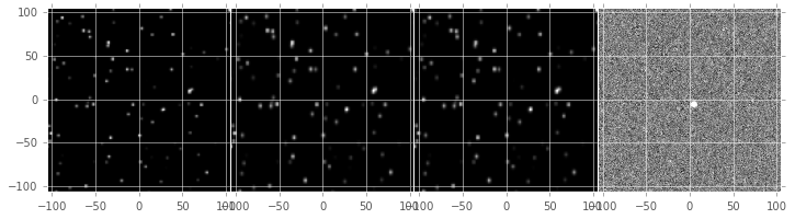
Figure 1 From left to right, sample (simulated) template image, PSF-matched template, science image, and difference image. In this simulated example, the source near the center was set to increase in flux by 2% between the science and template images.

In Figure 2 and Figure 3, we show the PSF matching kernel (\(\kappa\)) that was estimated for the images shown in Figure 1, and the resulting decorrelation kernel, \(\psi\). We note that \(\psi\) largely has the structure of a delta function, with a small region of negative signal, thus its capability, when convolved with the difference image, to act effectively as a “sharpening” kernel.

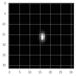
Figure 2 Sample PSF matching kernel \(\kappa\) for the images shown in Figure 1.

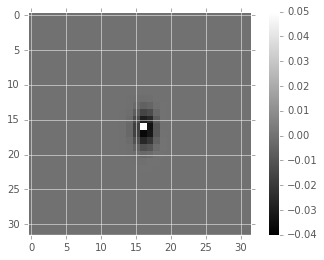
Figure 3 Resulting decorrelation kernel \(\psi\) (right) for the images shown in Figure 1.

When we convolve \(\psi\) (Figure 3) with the raw image difference (Figure 1) panel), we obtain the decorrelated image, shown in the left-most panel of Figure 4. The noise visually appears to be greater in the decorrelated image, and a closer look at the statistics reveals that this is indeed the case (Table 1, Figure 5, Figure 6, and Figure 7). Figure 5 shows that the variance of the decorrelated image has increased. Indeed, the measured variances (Table 1) reveal that the variance of the uncorrected image difference was lower than expected, while the decorrelation has increased the variance to the expected level:

In addition, we see (Table 1, Figure 6 and Figure 7) that the covariances between neighboring pixels in the image difference has been significantly decreased following convolution with the decorrelation kernel. The covariance matrix has been significantly diagonalized. While the covariance of the decorrelated image might at first glance appear high relative to the random expectation, we show (below) that it is equal to the value obtained using a basic implementation of the ZOGY proper image subtraction procedure.

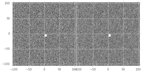
Figure 4 On the left is the decorrelated image difference, \(D^\prime\). Original image difference \(D\) is shown here for comparison, in the right-most panel, with the same intensity scale, as well as in Figure 1.

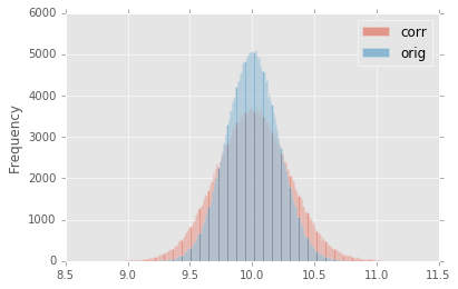
Figure 5 Histogram of sigma-clipped pixels in the original image difference* \(D\) (blue; ‘orig’) and the decorrelated image difference \(D^\prime\) (red; ‘corr’) in Figure 4.

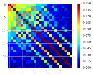
Figure 6 Covariance between neighboring pixels in the original, uncorrected image difference \(D\) in Figure 4.

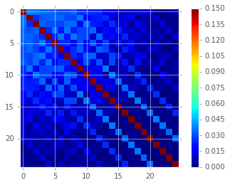
Figure 7 Covariance between neighboring pixels in the decorrelated image difference \(D^\prime\) in Figure 4.

3.2. Comparison with ZOGY.¶

We developed a basic implementation of the Zackay, et al. (2016) proper image differencing procedure (ZOGY) in order to compare image differences (see Appendix III. for details).

As shown in Table 1, many of the bulk statistics between image differences derived via the two methods are (as expected) nearly identical. In fact, the two “optimal” image differences are nearly identical, as we show in Figure 8. The variance of the difference between the two difference images is of the order of 0.05% of the variances of the individual images.

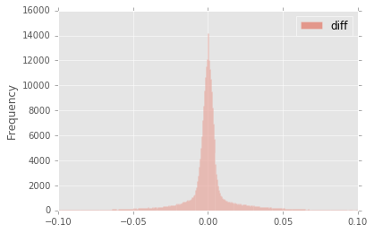
Figure 8 Histogram of pixel-wise difference between optimal image differences. Each image difference has been rescaled to unit variance to facilitate differencing.

3.3. Application to real data.¶

We have implemented and tested the proposed decorrelation method in the LSST software stack as a new lsst.pipe.base.Task subclass called lsst.ip.diffim.DecorrelateALKernelTask, and applied it to real data obtained from DECam. For this image differencing experiment, we used the standard A&L procedure with a spatially-varying PSF matching kernel (default configuration parameters). The decorrelation computation may be turned on by setting the option doDecorrelation=True for the imageDifference.py command-line task. In Figure 9 we show sub-images of two astrometrically aligned input exposures, the PSF-matched template image, and the decorrelated image difference.

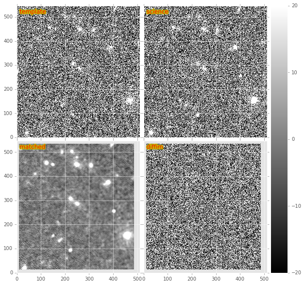
Figure 9 Image differencing on real (DECam) data. Sub-images of the two input exposures (top; template has been astrometrically aligned with the science image), the PSF-matched template (bottom-left), and the decorrelated image difference (bottom-right).

DecorrelateALKernelTask simply extracts the A&L PSF matching kernel \(\kappa\) estimated previously by lsst.ip.diffim.ImagePsfMatchTask.subtractExposures() for the center of the image, and estimates a constant image variance \(\overline{\sigma}_1^2\) and \(\overline{\sigma}_2^2\) for each image (sigma-clipped mean of its variance plane; in this example 62.8 and 60.0 for the science and template images, respectively). The task then computes the decorrelation kernel \(\psi\) from those three quantities (Figure 10 and Figure 11). As expected, the resulting decorrelated image difference has a greater variance than the “uncorrected” image difference (120.8 vs. 66.8), and a value close to the naive expected variance \(60.0+62.8=122.8\). Additionally, we show in Figure 12 that the decorrelated DECam image indeed has a lower neighboring-pixel covariance (6.0% off-diagonal covariance, vs. 35% for the uncorrected diffim).

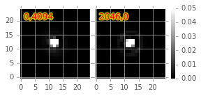
Figure 10 Image differencing on real (DECam) data. PSF matching kernels Shown are kernels derived from two corners of the image which showed the greatest variation in the matching kernels (pixel coordinates overlaid).

Figure 11 Decorrelation kernels corresponding to Figure 10.

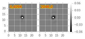
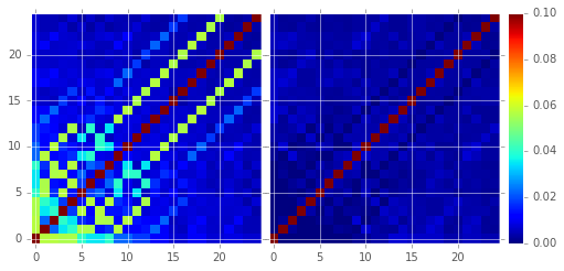
Figure 12 Image differencing on real (DECam) data. Neighboring pixel covariance matrices for uncorrected (left) and corrected (right) image difference.

3.4. Effects of diffim decorrelation on detection and measurement¶

See this notebook.

The higher variance of the decorrelated image difference results in a smaller number of DIA source detections (\(\sim\) 70% fewer) at the same default (5.5-\(\sigma\)) detection threshold (Table 2). Notably, if we decrease the detection threshold to the desired 5.0-\(\sigma\) level, the detection count in the decorrelated image difference does not increase substantially (\(\sim 14\%\)). However, the number of detections does increase dramatically (\(\sim 176\%\)) for the uncorrected image difference if we were to switch to a 5.0-\(\sigma\) detection threshold. (This is why the default DIA source detection threshold has previously been set in the LSST stack to 5.5-\(\sigma\)).

We matched the catalogs of detections between the uncorrected (“undecorrelated”) and decorrelated image differences (to within \(5^{\prime\prime}\)), and found that 45 of the 47 DIA sources detected in the decorrelated image are also detected in the uncorrected image difference. We compared the aperture photometry of the 45 matched DIA sources in the two catalogs (using the base_CircularApertureFlux_50_0_flux measurement) using a linear regression to quantify any differential offset and scaling. (We did not filter to remove dipoles, as the DipoleClassification task is still a work in progress and doing so would remove a large number of DIA sources. We found that there is no significant photometric offset between measurements in the two images, while the flux measurement is \(\sim 4.5 \pm 0.5\%\) lower in the decorrelated image. Unsurprisingly, the quantified errors in the flux measurements (base_CircularApertureFlux_50_0_fluxSigma) are \(\sim 120 \pm 5\%\) greater in the decorrelated image.

For a more thorough analysis, we recapitulated some of the work of Slater, et al. (2016), which described the issue with per-pixel covariance in A&L image differences generated by the LSST stack and the resulting issues with detection and measurement, but this time using the decorrelated image differences. With the help of Dr. Slater, we performed exactly his analysis on the same set of DECam images as described in Slater, et al. (2016). In Figure 13 below, we present an updated version of Figure 6 from Slater, et al. (2016) after decorrelation has been performed. We also present in Figure 14 and Figure 15 a version of Figure 7 from Slater, et al. (2016). Our analysis shows that the detections in the decorrelated image difference are now nicely tracking just at or above the \(5\sigma\) threshold.

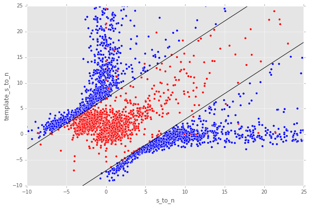
Figure 13 As in Figure 6 from Slater, et al. (2016): PSF photometry in the template and science exposures, forced on the positions of DIA source detections in the image difference following image difference decorrelation. The parallel diagonal lines denote science−template* \(>5\sqrt{2}\sigma\) and science−template \(< 5\sqrt{2}\sigma\), which are the intended criteria for detection. The numerous detections just at or below these detection thresholds have been eliminated, and (ignoring the two clouds of detections near (0, 0) and (-2.5, 2.5)) the primary detections are above (or below) the detection thresholds. Sources have not been filtered to remove false detections (e.g., dipoles).

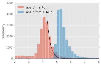
Figure 14 As in Figure 7 from Slater, et al. (2016): Comparison of force photometry SNR (red) versus the SNR in image difference (blue) for all sources in a single DECam exposure. The black line shows the expected detection counts from random noise (Slater, et al. (2016)). Shown here for uncorrected image difference (identical to Slater, et al. (2016)).

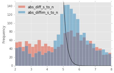
Figure 15 Same as Figure 14, but for sources detected at* 5-\(\sigma\) *in the decorrelated image difference.

4.1. Accounting for spatial variations in noise (variance) and matching kernel¶

There will be spatial variations across an image of the PSF matching kernel and the template- and science-image per-pixel variances (an example of the kernel variation is shown in Figure 10 and Figure 11). These three parameters separately will contribute to spatial variations in the decorrelation kernel \(\psi\), with unknown resulting second-order effects on the resulting decorrelated image. If these parameters are computed just for the center of the images (as they are, currently), then the resulting \(\psi\) is only accurate for the center of the image, and could lead to over/under-correction of the correlated noise nearer to the edges of the image difference. Another effect is that the resulting adjusted image difference PSF will also not include the accurate spatial variations.

We explored the effect of spatial variations in all three of these parameters for a single example DECam CCD image subtraction. The PSF matching kernel for this image varies across the image (Figure 10 and Figure 10), and thus so does the resulting decorrelation kernel, \(\psi\). Additionally, the noise (quantified in the variance planes of the two exposures) varies across both the template and science images by \(\sim 1\%\) (data not shown here, but see this IPython notebook). We computed decorrelation kernels \(\psi_i\) for the observed extremes of each of these three parameters, and compared the resulting decorrelated image differences to the canonical decorrelated image difference derived using \(\psi\) computed for the center of the images. The distribution of variances (sigma-clipped means of the variance plane) of the resulting decorrelated image differences differed by as much as \(\sim 5.6\%\) at the extreme (\(\sim 1.3\%\) standard deviation). The per-pixel covariance in the resulting images varied by as much as \(\sim 50\%\) (between \(4.0\) and \(8.0\%\)) at the extreme (\(\sim 25\%\) standard deviation) but all represented significant reductions from \(34.9\%\) in the uncorrected image difference. Finally, the number of detections on the image differences varied by \(10\%\) at the extremes (\(2.2\%\) standard deviation) around \(\sim 50\) detections total. We have yet to investigate DIA source measurement, which could be affected by the assumption of a constant PSF across the image difference.

We have not determined whether this uncertainty in image difference statistics arising from using a single (constant) decorrelation kernel and constant image variances for diffim decorrelation will have a significant effect on LSST alert generation. It is clearly at most a second-order effect, with measurable uncertainties of order a few percent at most. If this uncertainty is deemed to high, then we will need to investigate computing \(\psi\) on a grid across the image, and (ideally) perform an interpolation to estimate a spatially-varying \(\psi(x,y)\).

4.2. DIA Source measurement¶

The measurement and classification of dipoles in image differences, described in Reiss (2016) is complicated by image difference decorrelation, because dipole fitting is constrained using signal from the “pre-subtraction” template and science images, as well as the difference image. The prior assumption (for uncorrected image differences) has been that the PSF of the difference image is identical to those of the science and pre-PSF-matched template images, and thus the science image \(I_1\) could be reconstructed from the difference image \(D\) plus the PSF-matched template image \((\kappa \otimes I_2)\):

The decorrelation process modifies the PSF of the image difference such that this equivalency no longer holds, and the PSFs of the three images are now different. We will need to update the DipoleFitTask to accurately model dipoles across the three images. However now that the noise is accurately represented in the variance plane of the decorrelated image difference, dipole measurement should be more accurate and covariances will not be a concern.

5.A. Appendix I. Technical considerations.¶

1. A complication arises in deriving the decorrelation kernel, in that the kernel starts-off with odd-sized pixel dimensions, but must be even-sized for FFT. Then once it is inverse-FFT-ed, it must be re-shaped to odd-sized again for convolution. This must be done with care to avoid small shifts in the pixels of the resulting decorrelated image difference.
2. Should we use the original (unwarped) template to compute the variance \(\sigma_2\) that enters into the computation of the decorrelation kernel, or should we use the warped template? The current implementation uses the warped template. This should not matter so long as we know that the variance plane gets handled correctly by the warping procedure.

5.B. Appendix II. Derivation¶

Starting with the A&L expression,

where \(I_1\) is the science image with PSF \(\phi_1\). The model is that the true sky scene \(D\) is convolved with \(\phi_1\), so if we assume Gaussian, heteroschedastic noise (sky noise-limited), take a Fourier Transform, and compute the log-likelihood, we obtain

Then the MLE for \(D(k)\) is

with noise having variance

The variance diverges at large \(k\) as \(\phi_1^2(k)\) approaches zero, but (as shown by Kaiser (2004) and Zackay, et al. (2016)) we can flatten the noise spectrum (“whiten the noise”) to obtain the expression in (1), which we will repeat here:

To compare this calculation to the ZOGY expression, we take the ZOGY assumption that \(\phi_1\) and \(\phi_2\) are known, and thus \(\kappa(k)=\phi_1(k)/\phi_2(k)\). Substituting this into (1) gives us:

which is identical to Equation (13) in Zackay, et al. (2016), (3) below, except for an additional factor \(\sqrt{\overline{\sigma}_1^2 + \overline{\sigma}_2^2}\).

5.C. Appendix III. Implementation of basic ZOGY algorithm.¶

We applied the basic Zackay, et al. (2016) procedure only to a set of small, simulated images. Our implementation simply applies Equation (14) of their manuscript to the two simulated reference (\(R\)) and “new” (\(N\)) images, providing their (known) PSFs \(P_r\), \(P_n\) and variances \(\sigma_r^2\), \(\sigma_n^2\) to derive the proper difference image \(D\):

Here, \(F_r\) and \(F_n\) are the images’ flux-based zero-points (which we will set to one here), and \(\widehat{D}\) denotes the FT of \(D\). This expression is in Fourier space, and we inverse-FFT the image difference \(\widehat{D}\) to obtain the final image \(D\).

def performZackay(R, N, P_r, P_n, sig1, sig2):
    from scipy.fftpack import fft2, ifft2, ifftshift

    F_r = F_n = 1.  # Don't worry about flux scaling here.
    P_r_hat = fft2(P_r)
    P_n_hat = fft2(P_n)
    d_hat_numerator = (F_r * P_r_hat * fft2(N) - F_n * P_n_hat * fft2(R))
    d_hat_denom = np.sqrt((sig1**2 * F_r**2 * np.abs(P_r_hat)**2) + (sig2**2 * F_n**2 * np.abs(P_n_hat)**2))
    d_hat = d_hat_numerator / d_hat_denom

    d = ifft2(d_hat)
    D = ifftshift(d.real)
    return D

We note that we can also perform the operation in a way that allows us to avoid FT-ing the images directly. This involves computing two convolution kernels in \(k\)-space, convolving each of the two images, and then subtracting. If we define two convolution kernels \(\zeta\) and \(\eta\) such that:

then we can iFFT \(\widehat{\zeta}\) and \(\widehat{\eta}\) and compute

We have performed this calculation and we obtain identical image differences to those computed using (4), above.

5.D. Appendix IV. Notebooks and code¶

All figures in this document were generated using IPython notebooks and associated code in the diffimTests github repository, in particular, notebooks numbered 14, 13, 17, 19, and 20.

The decorrelation procedure described in this technote are implemented in the ip_diffim and pipe_tasks LSST Github repos.